In late 2015, TMR commissioned TransPosition to develop and test a series of potential scenarios for the introduction of Autonomous Vehicles (AV) into South-East Queensland (SEQ). The work found that connected and autonomous vehicles will lead to significant changes in mode share, total travel demand, congestion and road safety outcomes. This work had a particular focus on the impacts, opportunities and interactions between AV’s and traditional and innovative public transport services. In addition to proving better context for making current business decisions, there are a number of innovative approaches to the provision of public transport that are being considered; some of these are enabled by the same technology that underlies autonomous cars. These include the provision of Demand Responsive Transport (DRT) and Mobility as a Services (MaaS).
Following on from this work Transposition investigated the operational characteristics of various shared autonomous services for a selected set of scenarios using a new operational micro-simulation model. For this we have preliminary results of a number of areas in SEQ, and are currently in the process of extending over a wider area and finalising interactive animations that display the operation of a fleet of AV that collect passengers on demand and deliver them to their closest Bus (BUZ and CityExpress) or Train station.
Autonomous feeders to public transport
Autonomous feeders are intended to ensure that the autonomous services complement the mass transit offering rather than directly competing, and are assumed to involve government subsidy. Because of these facts it is important to ensure that they do provide a non-competing service while still opening up improved connections to public transport. This is more difficult than it initially appears.
To understand this, it is useful to consider the different types of travel that are available in the model. Unscheduled modes allow unconstrained travel through the network, where people can choose the routes that maximize their own utility. These modes include driving, walking and cycling. Scheduled modes only allow travel along particular routes and at particular times. People can freely travel to these services, but are constrained on when they can board and where they will be taken.
Our first attempt at modelling autonomous feeders was to treat them as an unscheduled mode with no constraints on when people could start using an AV feeder, but limits on where they could get off and what modes they could transfer to. Under these assumptions the model simply needed to ensure that anyone using the AV feeder would do so as part of a multi-modal PT trip. This approach worked, but gave results which were far from ideal. The model showed the very high use of the feeder services, but low public transport demand (as measured in passenger-km). Investigating the reasons for this it became clear that the AV feeder was too effect – people would travel on the feeder until they had almost reached their destination and then switch to public transport for a single stop to ensure that the trip was marked as PT. The most common destination for the AV feeder services was Roma St station, with people then transferring to buses or trains to travel a single stop (to Central Station or to the King George Square Bus Station). The model was doing what it was asked to do, but the service offering was poorly formulated.
It became clear that the AV feeder service needed to be constrained to an efficient set of origins/destinations and not allow people to travel arbitrary routes or long distances. A simple approach would be to limit the feeder service to just the closest public transport stop. However this seems overly restrictive – we want to ensure that the feeder service opens up new opportunities for public transport use, not overly constrain them.
The finally adopted approach was to draw on the closest Bus or Train station. Each location would have feeder services available to them that would take them to the closest stop for each of the defined network categories within reach. Because some modes (such as rail) are more likely to provide competitive services than the local bus services, the maximum catchment distance has been adjusted by mode. Most modes are constrained to 3km, with trains allowing a catchment of 5km. Ferries and non-CBD buses have a reduced catchment of 1.5km. The model was then used to consider each public transport network in turn. A modified path building process was used to find all network nodes within the maximum catchment distance of each station and record the travel times and distances. A loaded 2046 Base network was used to estimate congested travel speeds along the road network — for simplicity the PT feeder catchments are not adjusted between scenarios but are shared across all of them. The PT feeder services are then assumed to provide a direct transfer between that node and the stop/station, The following maps show a section of the resulting PT feeder network. The first map shows the area around central Brisbane (with The Gap and Chapel Hill in the west and Bulimba and Holland Park in the east). The longer distance train connections can be seen, as well as the shorter catchments for other route categories. Another important feature is obvious on the first map — the area around the CBD does not have any feeder options. This is because the modelling has assumed that anyone starting or ending their trip in the CBD will make direct use of PT (with walking access) rather than use a feeder service. This seems a reasonable constraint as it would be counterproductive to provide subsidized feeder services in the CBD itself.
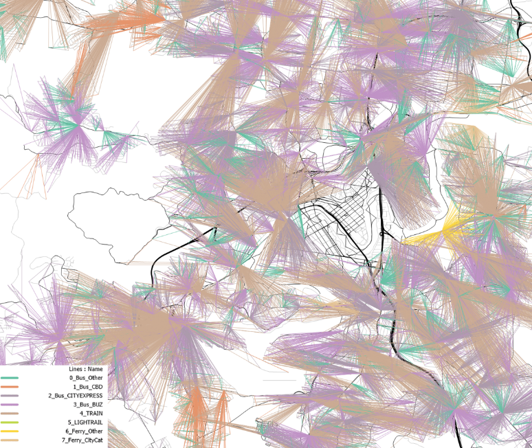
PT feeder network in area around central Brisbane
The full set of feeder alternatives is even clearer on the second map, which shows the detail west of Brisbane CBD in the area around Bardon. A single site (at the end of Bowman Parade) has been highlighted to show the alternative feeder options at that location.
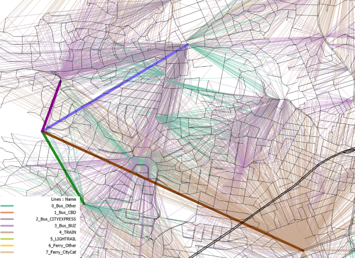
Pt feeder Network in the area around Bardon. A single site at end of Bowman Parade) shows the alternative feeder options at that location.
4S model Scenario
The microsimulation looks at the operation of the Autonomous feeders to public transport. This demonstration uses 2046 demographics and assumes the current PT services available on the SEQ GTFS feed. This scenario assumes that car ownership reduces as described by the autonomous vehicle ownership model, and that hired autonomous vehicles (autonomous taxis and autonomous carpool) are using the following parameters in the model
- Time Cost: 15c/min
- Distance Cost: 40c/km
- Flagfall: $1.20
- Wait time: 2-5 min (triangular distribution with a peak at 3 minutes)
- Time weight: 1.0
The outputs of the 4S model produce the trip demand (i.e. number of PT feeder trips) and the overall congestion on the network, these outputs are then fed into the microsimulation.
The figure below shows the volume (number of people) of people dropped off or picked up by a PT feeder at each PT stop. In the figure you can see the area that the Pt feeders are not allowed, this area exclusion has resulted in the largest PT feeder stops being along the areas neighbouring the exclusion zone. This is due to people trying to optimise there route to get as close to the city as possible before catching PT, so they may only be on the PT service for one stop.
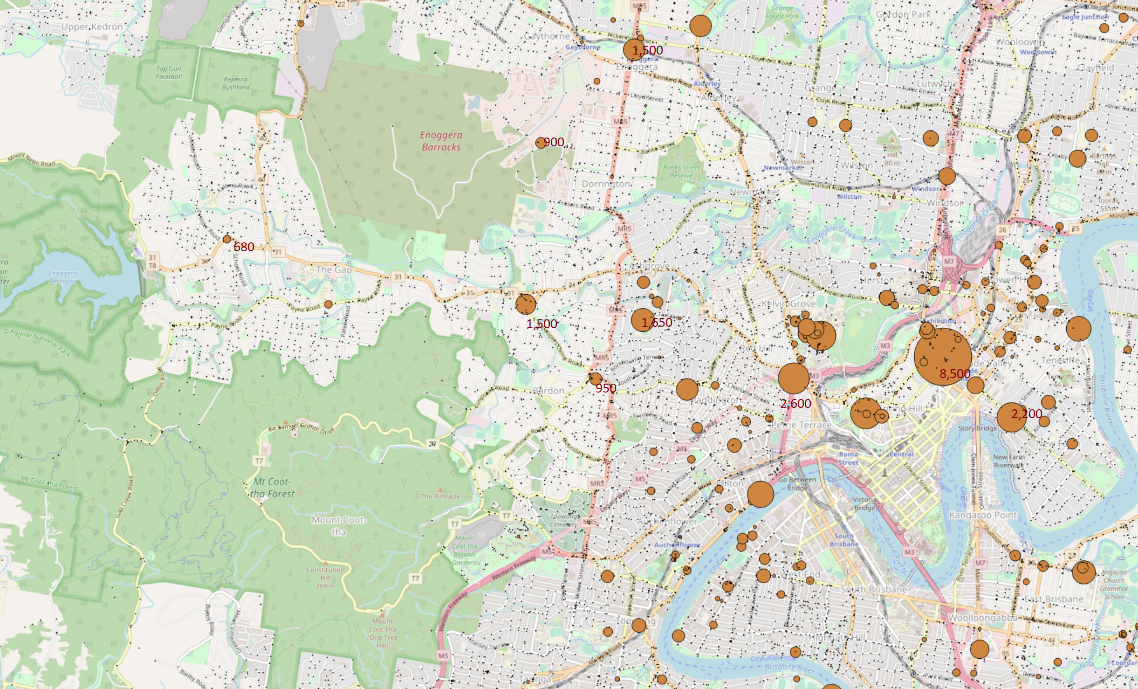
All day volumes at Origin to Pt Feeder locations
The volumes on the SEQ network generated by the 4S model in 2046 when assuming the Optimal Pt scenario is shown below. The shared (blue) volumes show the Pt feeders, from this map we can see that private vehicles still dominate the network.
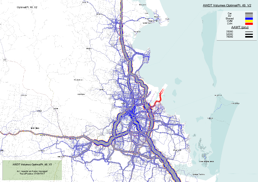
Traffic volumes across the SEQ network
Microsimulation
Details of how the microsimulation work to be added
Preliminary Results
Using the 4S model outputs described above we run the microsimulation model to determining the operation of a fleet of AV that collects passengers on demand and delivers them to their closest Bus (BUZ and CityExpress) or Train station. Due to the complexity of this we first look at how the AV fleet might operate over a smaller area. The results of this preliminary investigation are shown in the following section.
Model area
This simulation was run over the SA3 areas called The Gap – Enoggera and Brisbane Inner – West, as shown below. In 2046 this area is forecasted to have the following demographics:
- Population of 150,000
- 85,000 works will reside in that area
- Will be 8,100 FTE tertiary education enrolments
- 30,200 school enrolments
- The area will employ 91,000 people
- Across the area there will be about 40% private AV ownership, 52% Private AV non-ownership (any veh)
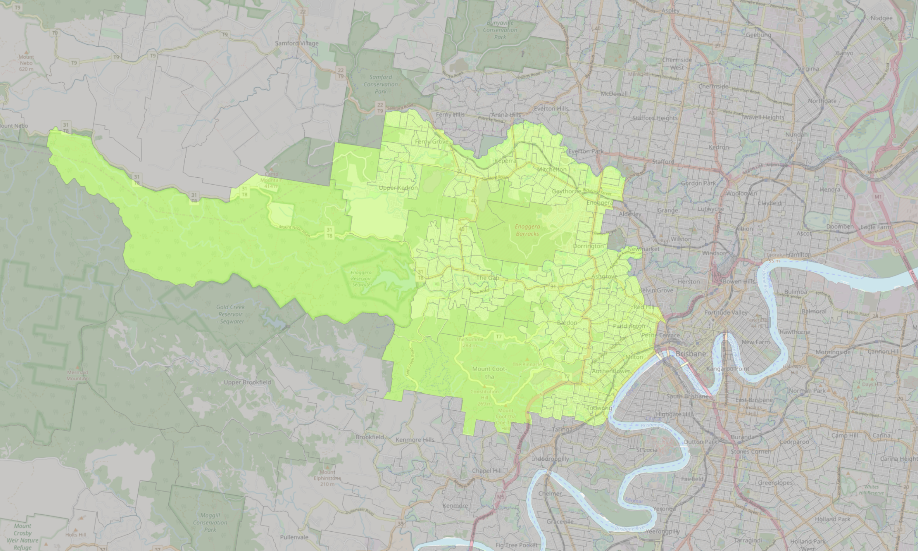
Modelling areas: The Gap - Enoggera and Brisbane Inner - West
Outputs
In deciding the operation of the Pt fleet there are several input parameters that can be varied. The most influential one is the number of vehicles in the PT fleet. Other parameters that could be varied are:
- maximum wait time before a passenger cancels a trip (currently set to 30 minutes),
- amount of time a passenger expects a pick up to take after notifying their trip (currently set to 3 minutes),
- if no vehicle is available to collect a passenger the trip will be delayed for 5 mins and then a new notification will be sent.
Currently the model looks to optimise each individuals route, to do this we also set a maximum permissible delay (MPD). This delay sets the length of time an individual is allowed to be delayed, when picking up additional passengers. In this preliminary investigation we look at the effects of changes in the size of the vehicle fleet and the maximum permissible delay.
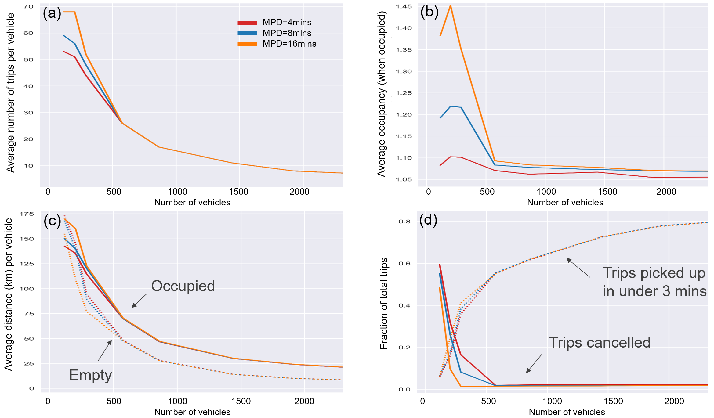
Figure (a) below shows the average number of trips done by each vehicle throughout a day (24 hour period), while (d) shows the average distance travelled for each vehicle whilst empty and occupied. Not surprisingly we can see that as the number of vehicles increases each vehicle does a smaller number of trips and thus travel a shorter distance. After about a fleet of 1,000 vehicles, the change to the number of trips and distance travelled becomes less significant. The number of trips and distance does not seem to be very sensitive to the maximum permissible delay. After a fleet of 600 vehicles the effect of changing the MPD is no longer visible when looking at the averages across an all-day time period.
MicroSim output plots
When the fleet is very small (100-200 vehicle) the increased delay allows more trips to be collected, this is likely due to passengers being inconvenienced for longer as additional passengers are collected, rather than the trips being cancelled. This can be seen in (b) where the average occupancy with a fleet size less then 600 is significantly higher when the MPD is 16 minutes. When a fleet has more then 600 vehicles the trips are nearly always singles occupant, regardless of the MPD.
Figure (d) shows that for close to no trips to be cancelled for MPD of 4 minutes at least 600 vehicles are needed, however with an MPD of 16 minutes, all trips can be collected with only 300 vehicles. This figure also shows that, unsurprisingly, the larger the fleet the more trips can be collected in under 3 minutes, at the expense of vehicle efficiency.
The figure below also highlights the benefit of having a longer MPD when fleet sizes are around 300 vehicles, in the figure you can see that the pick-up delay averages ~6min and the drop-off delay averages 8mins, where as a MPD of 4 mins results in a 9 min average pick-up and drop-off delay. This variation in delay happens when vehicles are in short supply, and thus it’s quicker to use a nearby occupied vehicle and add travel time to the passenger already occupying the vehicle. This shared occupancy results in the average time for all passengers being reduced. This effect can also be seen in the gap between the pick-up delay and drop off delay that does not exist for the other MPDs and in the spike in average vehicle occupancy for 300 vehicles and 16 minute MPD in Figure (b).
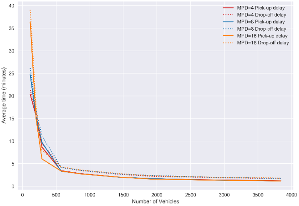
Average pick up and drop off for passengers
The daily operation (over 24 hours) of a vehicle fleet can be broken up into a number of vehicle events:
- waiting empty for a trip notification,
- moving empty to a pick-up point,
- waiting for passengers to get in and out of a vehicle,
- moving with a single occupant to a drop-off point,
- moving with multiple occupants to a drop-off point.
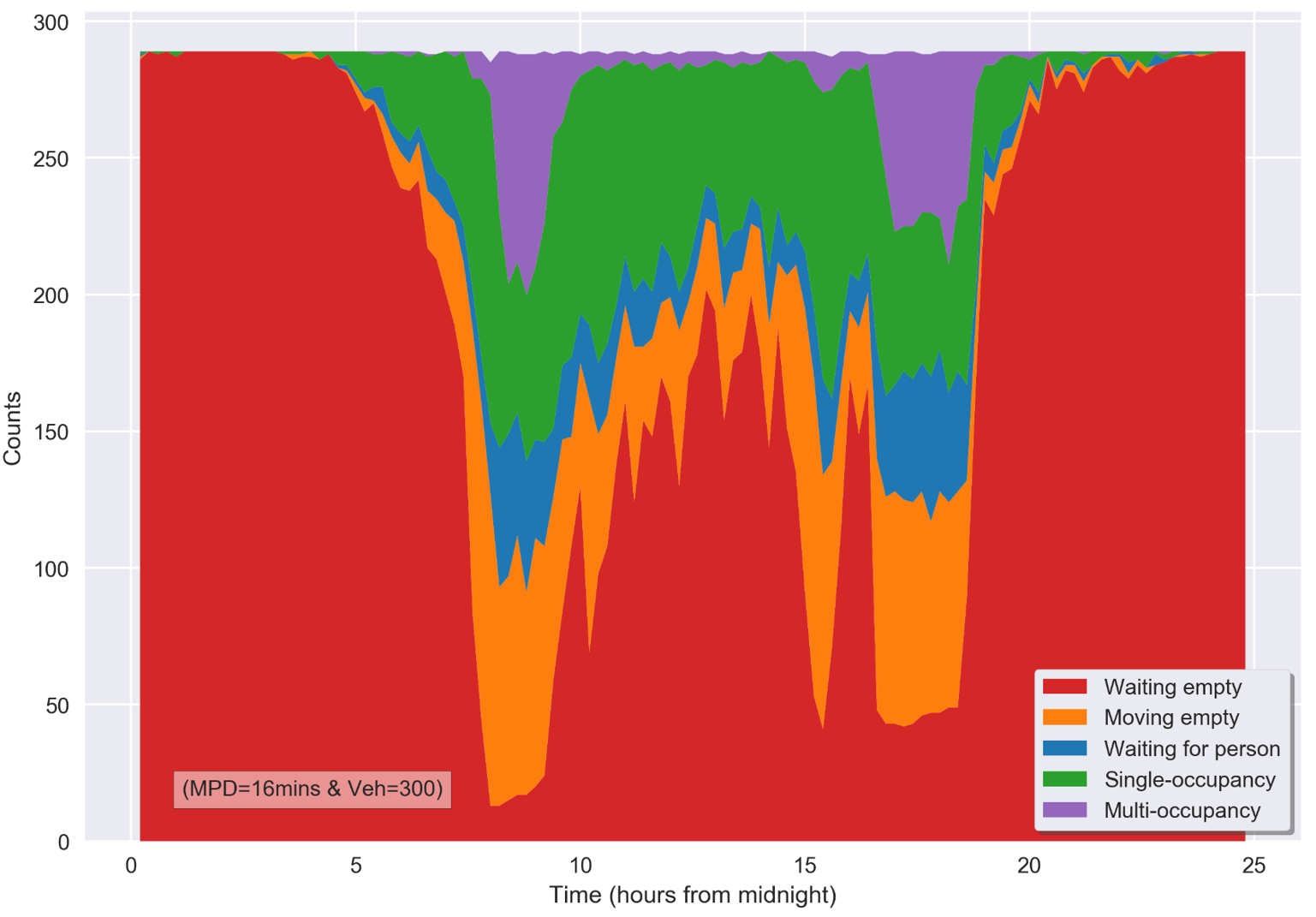
To gain an idea of the daily vehicle event time profile we look at a fleet of 300 vehicles and 16 minute maximum permissible delay, as this combination results in significant multi-occupant trips. The vehicle event time profile is shown below.
Fleet efficiency
The plots clearly show the AM and PM peak demand and that during the peak demand is when the vehicle contain multiple occupants. One of the effects highlighted by the vehicle event plots is the significance of the vehicle wait times while picking up and dropping off a passenger. The plots show that during the peak period around 15% of vehicles are waiting for passengers. Currently the waiting times allowed in the model are 60 seconds for people to get in a vehicle and 20 seconds for them to get out. These times were chosen as a starting point, that we believed was both generous and realistic. However, these results show that if multi-occupancy trips are to become more effective a method of reducing these times will be essential.