
The model is based on travellers making decisions that maximise their net utility. The net utility is the utility of their chosen activity at their chosen destination, minus the cost of travelling to that destination. As is usual for utility models, a generalised cost approach is used. A generalised cost approach endeavours to convert all components of travel impedance into dollar cost values. There are three main components of generalised cost; the value of the time spent travelling, the costs of operating the vehicle (including fuel cost, maintenance etc); and any other costs (including fares, tolls, parking etc).
There are a number of key, high level assumptions that the model makes about travel behaviour.
- Utility maximisation: People make decisions to maximise their overall net utility – that is the utility of the activity they can undertake at a destination minus the cost of travel to that destination.
- Random utility theory: People make different assessments of utility, so utility can be described by a random variable. In practice, this means that variables like walking speeds, wages, preferred arrival time, and perceptions of different destinations are all described with random variables.
- Generalised cost: People assess costs by adding up all of the components of their travel, including the weighted value of time spent travelling, vehicle operating costs, tolls, fares and parking charges.
- Behavioural factors constant over time: The determination of the key parameters that describe behaviour is done using current and historical surveys, and calibration against observed travel. In preparing forecasts, we change only those variables that are intended to change (such as population, employment and network characteristics). The behavioural parameters are assumed to carry forward into the future. This assumption can be relaxed in scenarios, but is implicit in the use of a current model to make predictions.
- Demand determined by land use: The main locational factor that determines travel demand is classified population and employment.
All of the components to travel are described by random variables, which reflect the probability that they will take any given value. For example, the speed that people walk can be described by a truncated normal distribution with an average of 5 km/h, a standard deviation of 2 km/h, and a minimum of 2 km/h. This means that people will typically walk at around 5 km/h, and very few people will walk faster than 9 km/h. Similar distributions can be set for all other variables that influence travel behaviour.
The key type of variables include:
- Cost elements: Value of time, walking speed, cycling speed, parking time and cost, vehicle operating costs, fares and tolls.
- Destination utility: the benefit of travelling to a given location (as opposed to an alternative destination) which is a function of the type of trip that is being considered, and characteristics of the destination (primarily size/number of jobs).
- Preferred arrival/departure time: the probability distribution of when people want to arrive at their attraction and when they want to leave.
For many choices, particularly the choice between modes and the decision on whether or not to use a toll road, the value of time is a key variable.
A worked example
A simplified example of the sort of calculations that the model performs can be seen in @fig:simplified-example. In this example, someone is wanting to travel to a medical service. They have 3 choices (in reality the model may consider thousands of alternatives) and they mentally ascribe dollar utility values to each of these choices. These values are unique to them, and a taken from random distributions based on what is available at each alternative (usually some measure of size, such as number of jobs). They also have a number of alternative ways of travelling to each destination, considering different routes and travel modes. Each of these different options are costed using the preferences specific to that person — including their value of time, mode preferences and time of day. The person is assumed to make the choice of destination, mode and route that maximises their net utility, which is simply the attractiveness of the destination minus the cost of getting there.
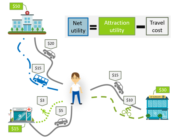
Simplified choice example
So in the example they have the following alternatives:
- Hospital, drive = $50 - $20 = $30
- Hospital, bus = $50 - $15 = $35
- Pharmacy, walk = $15 - $3 = $12
- Pharmacy, drive = $15 - $5 = $10
- Surgery, drive = $30 - $15 = $15
- Surgery, ride = $30 - $10 = $20
So in the example shown, the net utility is maximised if they catch the bus to the hospital, so that is what this person would do. At this point in the modelling the full detail of the trip is known, so the model can allocate the demand to the route at the time that the person is travelling. This enables the model to update its estimates about traffic congestion, public transport capacity etc.
Another person at a different location might have the same view of the utility values but would have different costs. The model efficiently explores the cost values at every location for a given set of preferences. This is why it is called an agent cloud — the model considers not just one agent, but a cloud of agents all spread across the city. Each “slice” of the model considers a new type of agent, with particular values of the attraction utilities, and and particular weights for value of time and mode preferences. This agent is then considered simultaneously at every location in the city, and their contributions are aggregated based on the likelihood that the agent would actually be at that location (using the specific market segment population).
Value of time
How to measure value of time
The value of time is a somewhat curious concept, because people have no ability to control how much time goes past – it is inexorably spent at the rate of 1 second per second. The only choice is what we spend our time doing, and so the value of time can only be understood as an opportunity cost; the value of time is the loss that we experience by doing something we would prefer not to do in contrast to doing something else. Since most people would rather not spend time travelling, the value of time is the amount that a traveller would be willing to pay in order to save time (Willingness to pay or WTP). When examined this way, it is clear that it is not possible to define a single value of time, since the value of time depends on how much the traveller likes or dislikes the time that they spend in a given activity. It also depends on how attractive is the next best alternative for their time use.
It is difficult to determine people’s value of time, since it cannot be directly observed. Some level of inference must be made, generally based on two sources of information. Revealed preference (RP) data looks at the decisions that people have actually made, and seeks to understand them in the context of trade offs between different alternatives. Stated preference (SP) data is obtained by asking people what choice they would make from a series of hypothetical alternatives. SP data is often preferred by modellers, because it gives a great deal of flexibility in presenting choices to people, and a wide range of values can be explored very quickly. Furthermore a single survey subject can be presented with many hypothetical choice experiments in a single session. In contrast RP data can only be found for choices that exist in the real world, and generally each subject can only provide RP data on a small set of choices; many times only a single choice is considered.
The flexibility of SP surveys comes at a very significant cost – they only look at people’s hypothetical choices, not their actual choices. Thus the surveys rely on people being good at imagining different alternatives and making choices that would reflect what they would actually choose if presented with those choices in real life. The difficulty that exists for all SP surveys is compounded when they are used for valuing travel times on toll roads. This is because the choices that are presented inevitably describe the alternatives by sets of numbers – for example, the travel time on the toll road, the travel time on the free road, the toll price. For people to accurately assess these alternatives they need to be good at hypothesising about sets of numbers, something with which many people have difficulty.
This problem is compounded when the surveys have an obvious real-world application. People will naturally try to understand why the survey is being done, and modify their answers to give an outcome that they desire, or to reflect values that they have. For example, people may seek to understate the willingness to pay for a toll road if they think that it will influence how the tolls are set. Alternatively they may overstate their willingness to pay if they want the road to proceed. We have anecdotal experience with truck drivers who stated that they would be willing to pay $50/trip for a new road before it had been committed, but then stated that they would not be willing to pay more than $20 once construction had commenced.
For these reasons, we are suspicious of the results from stated preference surveys and prefer first principles approaches, tested against revealed preference data. There are two key sources for revealed preference data – the household travel survey, and traffic counts on the tolled facilities. The household travel survey is based on surveys done by thousands of households every year. Each household is asked to report all of their travel on a single day.
We have made extensive use of both of these sources to prepare a realistic revealed preference approach. The approach that we have used is predicated on the assumption that people’s opportunity cost of time use is fundamentally related to their income. While not everyone has the ability to directly substitute their time for additional income, the rate at which people are compensated for engaging in work is a good starting point for their valuation of other uses of time.
Factors used in the model
The core idea in the model is that the value of time spent in travelling is made up of three components.
- The basic underlying rate (the wage rate), which varies between individuals but also varies between groups (e.g., working adults will have a different basic rate than students).
- A factor based on the purpose/type of trip (e.g., going to work vs going shopping).
- A factor based on the type of travel being undertaken (e.g., spending 10 minutes on a train c.f. spending 10 minutes walking).
Note that the wage rate is used as an input even for those who do not receive wages (such as children), since it assumed that their time is still correlated with wages, albeit with a lower factor. Note also that these variables (particularly the basic wage rate) will vary between individuals, and this will be captured through the Monte Carlo analysis. They may also change for a single individual over time or over different decisions. The underlying variability in the rate does not distinguish between the difference between individuals and the differences over time – the variability will capture both of these effects.
The distribution of earning across the community is commonly modelled using one of three possible distributions: exponential, gamma and log-normal. In this model the log-normal distribution has been used. The probability density function for a log-normal distribution is given by:
\displaystyle P_X (x)= \frac{1}{x \sigma \sqrt{2 \pi} } e^{\frac{-(\ln x - \mu)^2}{2 \sigma ^2}}, \quad x>0.
Where x is a specific value taken from the range of all values that the random variable, X, can take (in our case x can be interpreted as the hourly income); and \mu and \sigma are the input parameters which can be defined through the relationships for the mean and median below:
\displaystyle \text{Median} = e^{ \mu } \quad \text{and} \quad \text{Mean} = e^{\mu + \frac{\sigma^2}{2} }.
The input parameter, \sigma used was 0.8 which was based on a study of the personal income distribution in Australia by Banerjee, Anand, Victor M Yakovenko, and Tiziana Di Matteo in 2006. This paper examined data collected by the Australian Bureau of Statistics (ABS) on personal income distribution in Australia for 1989—2000, and concluded that the \sigma value generally lies in a range between 0.7 and 0.8. We chose the higher value due to the trend for wages growth in recent years to be more heavily weighted towards higher incomes.
In this example the mean was based on the average weekly earnings (AWE) in Queensland in 2017 (taken from QLD official website) which was $1489.10. Assuming that 38 hours make up a typical work week, we then have average hourly earnings (AHE) of $39.19, which becomes our mean value. Given that, the formula for the mean can be re-written as:
\displaystyle {\mathrm Mean}=e^{\frac{\sigma ^2}{2}} \times {\mathrm Median} \approx 1.377 \times {\mathrm Median}.
The resulting hourly probability distribution is given below.
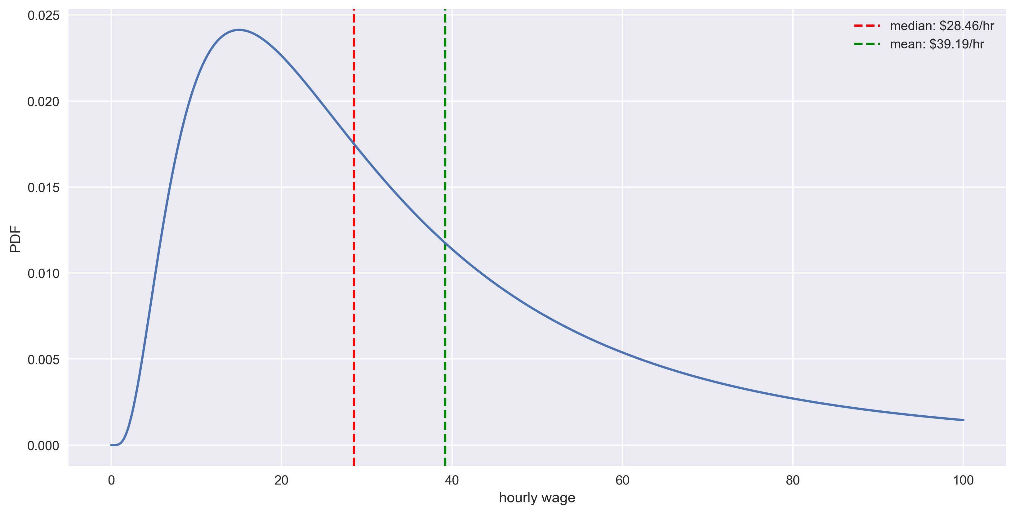
Log-normal probability distribution function based on wages
The basic wage rate is then factored for different person/trip types. The factors are as follows:
- worker (non-working time, e.g., commuting, lunch etc.): 0.6
- worker (working time): 1.3
- general non-work related: 0.5
- students: 0.3
- people travelling to the airport for personal reasons: 1.1
- people travelling to the airport for business: 1.4
These factors were developed using the household travel survey data. Consideration was also given to research done in 2002 by the Queensland University of Technology (QUT), “Modelling Tolls: Values of Time and Elasticities of Demand: A Summary of Evidence,” on travel time values and modelling approaches built on an international survey including Australia, USA, UK and other countries. The study found a multiplier of 40-50% times the average wage rate was widely accepted for non-business related trips (business trips refers to trips taken on working time). This paper also mentioned that the work related travel on working time tends to be valued higher with rates of 80-100%. We made the assumption that people travelling for work purposes generally rate their value of time somewhat higher than this since the lost time impacts on their overall productivity, not just their wages.
To allow for variability in traveller’s perception of the attractiveness of different modes, the basic value of time is further adjusted by mode-specific random variables. These values are unlikely to be completely independent — someone who dislikes public transport will dislike both buses and trains. For this reason the public transport time weights are the product of a common public transport weight and a mode specific factor.
Value of time for commercial vehicles
For commercial vehicles, the value of time includes a number of components — the value of the driver’s time, the opportunity cost of the vehicle, and the value of time of the freight itself. The wage of a truck driver is much less variable than that of a car driver; car drivers come from a very wide range of occupations and incomes, whereas almost all trucks are driven by people with the same occupation — truck drivers.
The value of time for commercial vehicles has been determined by assuming a spread to the hourly wages given in the Road Transport and Distribution Award and then adding some cost for the value of time of the vehicle and the freight itself. The wages vary by vehicle class, and assume a 38 hour working week. From July 20171
- for medium commercial vehicles (CVM), the relevant grade is Wage Grade 3 ($763.80/week = $20.10/hr)
- for heavy commercial vehicles (CVH) Wage Grade 7 ($808.20/week = $21.89/hr)
These wages are then increased by the same 1.3 factor that was used for working-time travel of car users. This reflects the on-costs and margins on the driver’s time.
The value of time of the vehicle and the freight is more difficult to determine. Some studies have used stated preference surveys to show that this factor is significant, but a highly variable based on the freight type (with the highest value for express, automotive and container loads, and the lowest value for bulk goods). An average rate for Australia in 1998 was found to be $1.40/pallet/hr.
Allowing for inflation (CPI July 2017=111.4, CPI July 1998=67.5) 2 this gives $2.31/pallet/hr. Assuming that a rigid truck carries 10 pallets and a semi-trailer has 20 pallets, and combination vehicles 35-50 pallets, this gives $23.10/hr for medium commercial vehicles and $46.21/hr for heavy commercial vehicles and $80.87-$115.50/hr for articulated/super-heavy vehicles. But note that this assumes that the vehicle is fully loaded — the model does not differentiate between the fully-laden trip and the return trip, so the average cost for freight should be reduced to allow for the proportion of dead running. Adding the corresponding numbers we get that the total rate (VOT) for CVM is $33.40 - $37.50/hr and for CVH is $45.70 - $64.03/hr.
Note that when this was implemented in the model we increased the effective VOT to allow for some portion of fixed costs3. Accounting for fixed costs is difficult, as it will depend on whether the drivers are supply constrained or demand constrained. If they are demand constrained then it may not be rational to price in a full allowance for fixed costs – saving time will not increase profits and will not reduce the fixed costs. However if they are supply constrained (i.e., they would need to buy new vehicles to increase their capacity) then saving time would reduce the need to incur new fixed costs. We have adopted an increased spread in the hourly cost to allow for this. Therefore the final VOT distributions used in the model were $45-$70/hr for CVM and $65-$90/hr for CVH. Note that the direct operating costs (fuel, tyres etc) are included in the distance-based operating costs, not in the time cost.
We model class 3 (CVM) and class 4 (CVH) vehicles using a linear distribution of the VOT instead of the log-normal distribution we used for class 1 and class 2. A linear approach was used for a number of reasons; firstly driver wages are generally fixed to a small number of awards and these put constraints on how low or high wages can be. Secondly, the time value of the freight itself is variable, but significantly impacted by the quantity of freight carried. Because the model has no assessment of whether commercial vehicles are empty or fully loaded, we use a linear distribution to reflect the range of loaded conditions between empty and full.
Parking cost and availability
As well as the costs that apply to links, and intersections, there are other costs that apply at the start or end of the trip. These include allowances for the time to park cars as well as the payment of any parking charges. Parking in many high demand areas is often limited and costly, and therefore adds significant cost, time and inconvenience to private vehicle travel. For this reason, the parking cost and availability were included in the TPACS model inputs. Unfortunately, the parking in most of these areas is complex, as it contains a mixture of street parking (free and paid) and car parks. The car parks provide an hourly rate, an all-day parking rate and a rate for monthly or yearly parking permit holders. The rates for the parking also varies between the different areas and parking companies.
The model makes assumptions about the rate of parking that applies to each travel market with a reduced multiplier to the daily parking rate for some segments (e.g., health related travel, work, shopping). This reflects the various discounts that typically apply to these sorts of trips. The model also puts an effective parking zone around all train stations, even though these locations often do have some limited free parking options — these costs reflect the difficulty of finding a park in these locations, as well as the cost of parking. Note that no information on parking supply has been coded at these locations.
Toll road prices
The cost of all toll roads, and any future toll roads is used in the Model. The model allows different toll prices to be applied for each Vehicle class. The model can also apply capped toll pricing schemes, distance based tolls or simple toll points. In addition to this the model can apply toll discounting schemes, as well as apply tolling increases or decrease for different modelling scenarios to test the effects of Toll pricing changes.
Vehicle operating costs
After time (and tolls) the next most significant contributor to cost is vehicle operating cost, which we assume is related to the cost of fuel and other costs (tyres, maintenance etc.). An allowance for capital costs/depreciation is also included, but weighted down for car travellers (since people seem to consider the cost of car ownership as a sunk cost and do not typically consider it in their choices, unlike commercial vehicle operators who generally have a better understanding of full costs).
It is likely that a large increase in fuel price will lead to a range of effects. There will be some decentralisation of travel (as people shift to closer destinations) and some mode shift to PT/active transport. It will also improve the attractiveness of free flowing conditions, as fuel use is lower per kilometre. Its effect on the SEQ roads would thus be mixed.
The baseline model assumes a fuel price that varies between 15 cents and 35 cents per kilometre. This distribution of cost was chosen to represent the range in vehicle fuel consumption, e.g., electric vehicles to large 4WD.
Public transport and AV/Taxi/Rideshare service fares
The model uses the real cost of the public transport fares for each state. For example in SEQ the cost of public transport was obtained from the TransLink website. 4 The fares are based on the number of zones travelled in a journey and the price varies depending on:
- concession entitlements
- off peak or peak times
- travelling to and from the Brisbane airport
- using a go card or ticket
The same fare system can be extended to test the effect of Mobility-As-A-Service or new fare systems can be added to look at alternative future PT and ride share pricing schemes. The model can applying pricing discount based on person type i.e. student, disabled or pensioners.
See http://www.freightmetrics.com.au/Calculators/TruckOperatingCostCalculator/tabid/104/Default.aspx for a useful tool to examine the costs experienced by truck operators↩