The road, walkway and cycleway network used for the TPACS model draws on OpenStreetMap.

OpenStreetMap provided many attributes including geometry, road names, speeds, and lanes, making up the majority of the base year network. This was extensively checked against Google Map’s satellite view and other research to make sure the network was up to date. As OpenStreetMap is open-source, quick edits of the map were made, when sections were not up to date or inconsistent with aerial photography. These edits could then be re-download and used to update the map to be used in the model. An example of OpenStreetMap and the extracted network data used as the input for the model can be seen below – the figure shows a section of the network in Sydney’s CBD but the same approach been used for all models.

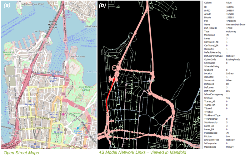
Imported OpenStreetMap data (a), coded into the 4s Model with road link attributes (b)

The key attributes extracted from the OpenStreetMap data are:

• road names and alignments
• number of lanes
• road type – which was used to determine hierarchy (1=Highway, 6=Residential Street)
• posted speed
• intersection types

Where the necessary attribute information was unavailable, a number of assumptions had to be made to prepare a network suitable for modelling. A hierarchy was assigned to each road based on its road type, speed, lanes and its urban/rural status. Based on these attributes road friction was also assigned. Friction can sometimes also be called traffic impedance, and is an overall measure of the degree to which traffic is constrained by side friction, road design standards etc. For example, Motorways would typically have very low friction while a local street would often have high friction.

SEQ Road Network

It is sometimes the case that OpenStreetMap does not include details on posted speeds and number of lanes. In these cases default values are used. The table below shows the default assumptions used for the Toowoomba network, the assumptions are adjusted to best reflect the area being modelled. The assumed free-flow speeds and number of lanes for a road are based on its hierarchy and metro/urban/rural location status. Note that the number of lanes is for a single direction — an entry of 1 in the table means a standard 2 lane road (with 1 lane in each direction). This convention makes the coding of one-way roads more consistent. These speeds reflect posted mid-block speeds; the delays at intersections are calculated separately.

Table: Regional city (Toowoomba) road assumptions based on hierarchy and urban/rural status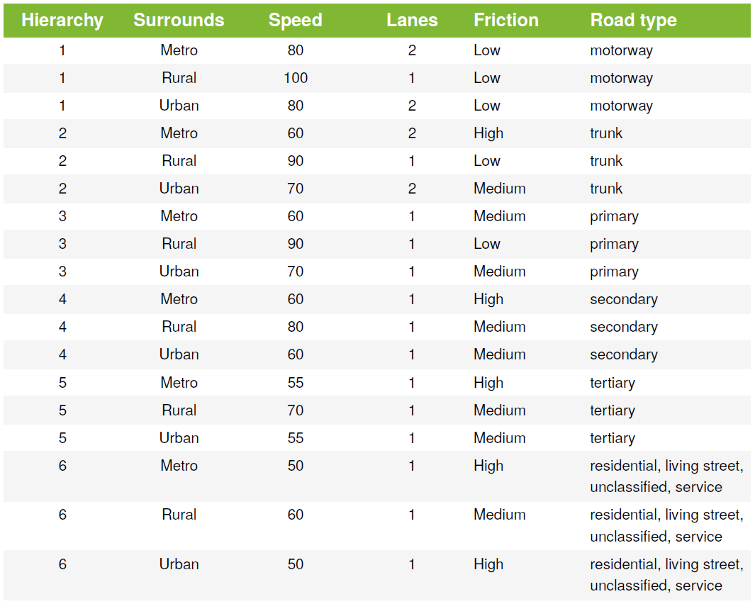

The road types given in table above are defined by OpenStreetMap¹ as follows:

• Urban areas:
  • Motorway: The metropolitan motorway network. ‘M’ classified roads in cities where they exist.
  • Trunk: Metroads or ‘A’ classified roads in the cities where they exist, or other similar cross-city trunk routes in cities where they do not.
  • Primary: Other main cross city and arterial routes. ‘B’ classified roads in cities where they exist. Major connecting roads in larger rural cities.
  • Secondary: Major through routes within a local area, often connecting neighbouring suburbs.
  • Tertiary: Minor through routes within a local area, often feeders to residential streets.
  • Residential: Residential streets.
  • Unclassified: Other streets. Not generally through routes.
  • Service: Un-named service and access roads. Also used for small named rear-access lanes.
• Regional roads:
  • Motorway: Motorways, freeways, and freeway-like roads. Divided roads with 2 or 3 lanes in each direction, limited access via interchanges, no traffic lights. Generally 100 or 110 km/h speed limit. For e.g., Hume Freeway. In states with the Alphanumeric system, these are ‘M’ roads if they are of freeway standard.
  • Trunk: National highways connecting major population centres. For example, the Bruce Highway north of Cooroy. State strategic road network, for example, Pacific Highway. In states with the Alphanumeric system, these are ‘A’ roads. ‘M’ roads which are not of freeway standard are also classified as a trunk road. In other states, these are signposted with a white National Road shield, or a Green National Highway shield.
  • Primary: State maintained roads linking major population centres to each other and to the trunk network. In states with the Alphanumeric system, these are ‘B’ roads. In other states, these are generally State routes signposted with blue shields.
  • Secondary: District roads that are generally council maintained roads linking smaller population centres to each other and to the primary network. In states with the Alphanumeric system, these are ‘C’ roads.
  • Tertiary: Other roads linking towns, villages and points of interest to each other and the secondary network.
  • Residential: Local streets found in and around cities, suburbs and towns as well as in rural areas.
  • Unclassified: Other named minor roads.
  • Service: Unnamed access roads, e.g., entranceways and roads in parks, government properties, beach access etc.

Information on off-road paths and tracks were also included, but only a subset was included in the model. The public transport network was implemented separately and is described at the end of the page.

Updating network information

The basic assumptions described above do not always apply, so the network information in the model was extensively reviewed, based on physical inspection and detailed examination in Google Earth, and StreetView. The review aimed to identify:

• Changes in the number of lanes
• Changes in posted speed
• Location and type of intersections
• Location and type of railway crossing and signalised pedestrian crossings

These changes were either updated directly into OpenStreetMap or coded as point based link transitions, which are a feature of the TransPosition modelling suite. They allow changes to network data to be specified with a point and a bearing. The points are snapped to the closest road that matches the bearing at that point, and then modify the data on that road in the direction specified by the bearing (see fig a in next section). This process makes it easy to see where basic network data in the OpenStreetMap layer has been overridden. It also means that the changes that have been made can be automatically applied to any updated version of the OpenStreetMap layer.

Future network options and improvements

A series of future network options have been identified and included in the 2036 model. Future network options can be coded into a geospatial database and associated with a specific option code; this allows the option to be included or excluded from a model run as required for the specified scenario. Changes to both existing roads and new roads can be coded.

Attributes of existing roads can be modified using point based link transitions (see figure a below). Some examples of characteristics of existing roads that can be changed are

• lane numbers
• posted speed limits
• degree of side friction (which influences speed and capacity)

Alternatively a new road can be added. This is done by drawing or importing the path of the new road using a Geographical Information System (GIS) and assigning all road attributes. Connection points are added where the road connects to the existing road network, see figure b below.

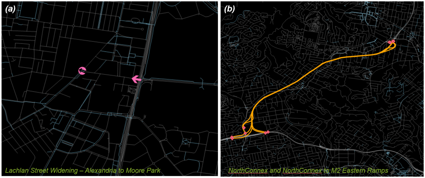
Option codes for future network changes—update an existing road with transitions (a) or add a new road (b).

Road capacities

Once the number of lanes and degree of side friction are determined, a separate table (@tbl:LaneCapacity) is used to assign hourly one-way capacities, and the Davidson J ² congestion parameter. The capacity of a single lane is dependent on the hierarchy, side friction, number of lanes, and whether or not the road is median divided.

The Davidson-Akcelik speed flow relationship is used

\displaystyle t = t_0 \bigg[ 1 + 0.25 r_{\text f}\bigg( z + \sqrt{z^2 + \frac{8J(1+z)}{r_{\text f}} } \bigg) \bigg]

where

• t = congested travel time
• t_0 = \text{free flow travel time} = \frac{ {\text length} }{ {\text uncongested speed} }
• z = \frac{ {\text volume} }{ {\text capacity} } -1
• r_{\text f} = \text{ratio of flow period to minimum travel time} = \frac{ T_{\text f}}{t_0}
• T_{\text f} = \text{duration of congestion: the model has assumed that } T_{\text f} = 1{\text hr}
• J is a delay parameter that determines how quickly a road congests as it approaches capacity. A road with a small J value will keep high speeds right up until close to the capacity, and then congestion will quickly increase. A road with a large J value will start to congest very early, and gradually deteriorate as flows increase. The J parameter is related to the level of side friction – generally the more friction there is the higher the J value will be.

The relation is shown below.

The Davidson-Akcelik speed flow relationship

Table: Lane capacities and the Davidson J congestion parameter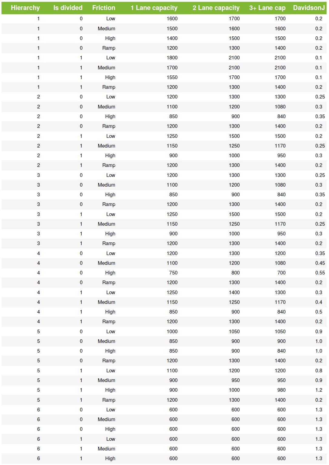

Public and active transport

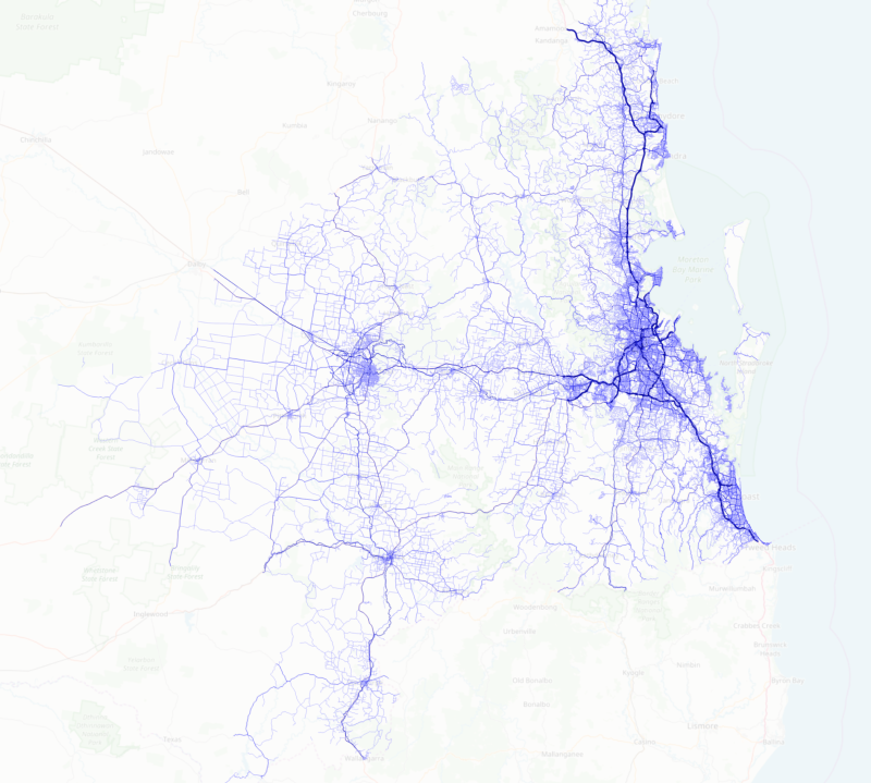
Public transport is the most significant alternative to private car use, particularly for travel to and from the CBD. The representation of the public transport network in the model is built from data provided by TransLink through their timetabling system. The information is provided in a standardised format – the General Transit Feed Specification (GTFS) ³. The GTFS format is used nearly world wide and available for all other states in Australia, additionally the model can combine GTFS feeds from different regions to model public transport across large regions. All regular scheduled services are included, with full time tables used by the model, however the model does not currently include school bus services. The stop locations were matched to points along roads and a composite multi-modal network was constructed. An example of a network in SEQ is shown below.

SEQ multimodal network

The Monte Carlo sampling used by the model includes a randomly selected arrival time (from the observed distribution for each travel purpose). When considering modes, the model will determine the best route and individual PT service to use. This means that the impact of travel time is implicitly incorporated — infrequent services will lead to long waiting times. To allow for the fact that people can plan their travel around public transport timetables, this first-stop waiting time is discounted. A random distribution is used for this to allow for the fact that people will have variation in their ability to reschedule their travel. The model also includes variation in people’s mode preferences (to account for the fact that some people are happy to use public transport and others are committed to cars) and weightings for different sub-modes (to reflect the general preference for ferries and trains over buses).

All major walking and cycling routes in the city are included in the model. The model also assumes that people can walk and cycle along all roads except for Freeway/motorways/busways. Different weights are used for off-road vs. on-road walking and cycling. The model allows for variations due to on-road cycling lanes but no data on this has been coded. As well as incorporating variation in people’s preference for walking and cycling (including variation in end-of-trip times) the model includes random variation in walking and cycling speeds. There are also factors for specific travel purposes — for example people are less likely to walk for shopping trips. For cycling, the model allows for time (and generalised cost) securing bicycles, showering (if necessary) and changing out of cycling gear.

The value of time, applies to all time spent travelling, with different weights for different experiences (e.g., walking time is weighted by 1.5; cycle time by 3.0; train time by 0.7 – 1.2; in car time by 1.0).