
The TPACS model uses an individual trip approach. Travel decisions are derived from activities by people categorised under different market segments, each having unique behavioural characteristics and undertaking activities in different geographical areas (e.g. work, school, leisure, commercial transportation).
This model approach addresses the shortcomings of the traditional Four-step model (FSM) such as:
- not recognising that travel is a derived demand
- assuming the travel decisions are made sequentially (where will I go/what mode will I take/what route will I travel)
- ignoring the significant variability in people’s travel behaviour, including their value of time and toll choice preferences (one of the causes of poor toll forecasting in traditional models)
- failing to properly address time of day; using separate peak and non-peak models rather than allowing time to be a continuous variable
Market segment assumptions
The model works with the concept of market segments, which are similar to the purpose breakdown in traditional models. But they are more generalised and allow for more detailed divisions of the travel market. A market segment represents a particular type of travel conducted by a group of people. The market segment can determine which modes are suitable; give distributions for value of time (or any other behavioural parameter); dictate the set of potential destinations; and select the appropriate population measure for determining the size of the market. One of the key differences between the TPACS model and other approaches is that the market segmentation is maintained throughout the model, even into path building and assignment. This allows the model to address the different ways in which people choose their preferred route, incorporating differences in value of time, toll preferences, and vehicle operating costs.
Private Travel Market Segments
The current implementation of the model uses a trip based (as opposed to tour based or activity based) approach and so, for example, trips from home to work are considered separately from trips from work to home. Thus another aspect of the market segment specification is the time-of-day preference. This is specified as a preferred arrival time for forward trips, and a preferred departure time for return trips. The market segments for private travel are similar to the purposes used in other models, but with a slightly more detailed breakdown. The model includes the following private travel market segments.
- HBW_Blue: Home Based Work (travel between home and work) for blue collar workers
- HBW_White: Home Based Work (travel between home and work) for white collar workers
- HBE_Prim: Home Based Education Primary School- travel to and from primary schools
- HBE_Sec: Home Based Education Secondary School
- HBE_Tert: Home Based Education – Tertiary education
- HBS: Home Based Shopping
- HBR_Social: Home Based Recreation (Social) – travelling to/from friends or family
- HBR_Commercial: Home Based Recreation (Commercial) – travelling to/from recreational activities
- HBO_Health: Home Based Other (Heath related) – travelling to/from doctors, hospitals etc
- HBO_Services: Home Based Other (Services) – travelling to/from personal business destinations
- WBW: Work Based Work – travelling between workplaces for work reasons
- WBS: Work Based Shopping – travelling to/from work to a shop, or stopping on the way to/from work
- WBO: Work Based Other - travelling to/from work to another destination, or stopping on the way to/from work
- SBS: Shopping Based Shopping – travelling between shops
- OBO: Other Based Other – travelling between other destinations
- WBO_SP: Picking up or dropping off people on the way to/from work
- HBO: Going from home to another destination, usually to pick people up or drop them off
- Air_Work: Airport related travel for business travellers
- Air_Private: Airport related travel for private travellers
The Person Type is used within the model to set a number of variables, including value of time distribution and applicable public transport fares. The Production parameter, along with the Trip Rate determines the number of trips that will be generated for that market segment. The model uses a simple person trip-rate generation model, with parameters taken from the Household Travel Survey. The Production variable gives the relevant demographic input, which is then multiplied by the specified trip rate.
The Attraction variable (along with the assumed distribution of the Attraction Utility random variables) determines what utility each potential attractor is given for a particular Monte-Carlo draw.
The relationship between utility and size is a little complex. It is generally the case that larger destinations will have higher utilities than smaller ones, but this is not always true – sometimes we will seek out a niche destination because it is particularly attractive. Furthermore, the attractiveness of a destination is not linear with size – we would expect a diminishing return as attractors get bigger. The basic logic used by the model is that each potential destination gives the traveller a number of opportunities to be satisfied, and the number of opportunities is proportional to the destination’s size (in this model, size is determined by employment numbers). The size of the destination is divided by the scale parameter to determine the number of opportunities. The utility of each opportunity is assumed to have a gamma distribution, with a specified mean and standard deviation. The utility of the destination is determined by taking a random draw from the gamma distribution for each opportunity, and then taking the highest value. In other words, the utility of an attractor is determined by the utility of the most attractive opportunity at that attractor.
This approach gives utility values that satisfy a number of features that we would expect utilities to have;
- The utility of an attractor is an increasing function of its size
- The marginal utility diminishes as an attractor increases in size, but is always positive (i.e. it does not asymptotically approach a fixed value, but keeps increasing at a reducing rate)
- The expected utility of two destinations at the same location is equal to the expected utility of a destination with a size equal to the sum of the individual sizes
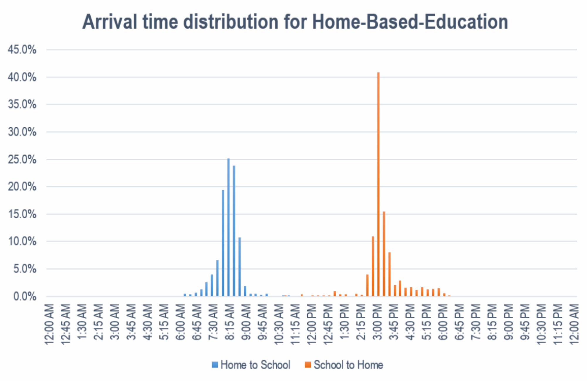
Each market segment has a time profile to determine what time of day the trips will occur. The production to attraction trip (e.g. home to work) is assumed to be fixed by preferred arrival time at the attraction. So if someone needs to get to work at 8:30am then they will leave at whatever time will get them to work on time. The attraction to production trip is assumed to be fixed by preferred departure time. At this stage there is no link between preferred arrival time and preferred departure time – the model treats them as separate random distributions. Because of the adding together of multiple slices in the Monte Carlo simulation, this lack of linkage is not a problem. Arrival time distributions have been determined by querying the Household Travel Survey to find actual arrival times throughout the day, grouped into 15 minute intervals. Separate distributions are set for trips from the home and for returning trips. There is undoubtedly some peak spreading already occurring in the network, so the pattern of actual arrival times is not the same as the pattern of preferred arrival times. It is difficult to determine how much people have modified their behaviour so the observed distribution is the best information available.
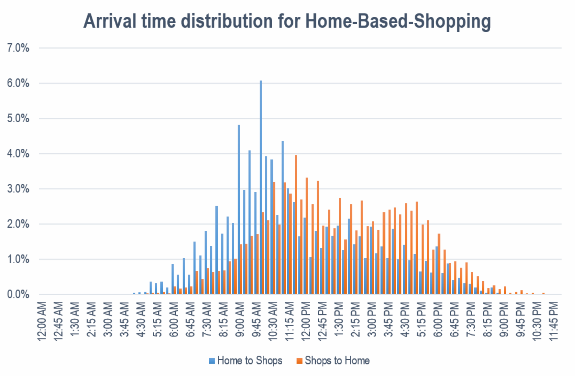
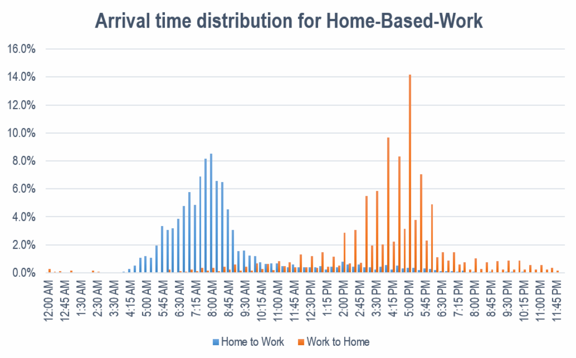
Some examples of the different types of arrival distribution can be seen in the following graphs. They show the distribution of From-Home and To-Home arrival times for Home-based-education (HBE), Home-based-shopping (HBS) and Home-based-work (HBW). It is clear that education trips are very peaked around school times, with some students arriving before school and some staying afterwards (with a longer tail in the evenings). People tend to travel to shops slightly after the morning peak (at 10am), and the peak time for going home again is 11:30am, but there are trips throughout the day. Work is somewhat similar to education, except that workers arrive earlier and stay later, and have a much wider spread. Significant numbers of workers get to work before 6am, and almost all have arrived by 9:30am, with a peak at 7:45am. Workers tend to leave work much more often on the hour or half hour than in other 15 minute periods leading to a sawtooth pattern to the work departure time. The peak time of departure is 5pm, with more workers leaving before this time than after.
Note that “serve passenger” trips are treated differently in this model than is often the case. Basically the driver for a serve-passenger trip is assumed to have subordinated their travel preference to the person who is being served. The purpose of the car’s trip is given by the purpose of the served passenger. Thus if a parent drives their child to primary school then this is a HBE_Prim trip. If they then drive on to work then this is a WBO trip. This approach is not entirely accurate, but “serve passenger” trip are inherently difficult and poorly modelled. This approach has the advantage of clearly showing the purposes of travel. A full treatment of this problem would probably require a tour-based or activity-based approach.
Commercial Vehicle (CV) Market Segments
The key idea is to represent the main industry linkages through separate market segments. The CV model uses 27 industry categories (e.g. Agriculture Forestry And Fishing is broken into Horticulture and Fruits, Grains and Meats, Dairying, Forestry and Logging, and Commercial Fishing). Usually employment forecasts are not consistent with this level of detail, so more aggregate industry groupings have to some times be used. The industry linkages are combined with estimates of Tonnes per Week per Employee (TWE) to give the estimated trip rates per employee. Assumptions are made on freight mode share by industry. National Input-Output matrices can then be used to link freight demand across industries.
Growth in Commercial Vehicles
The model determines the location and level of commercial vehicle demand based on employment in freight-related industries, the most significant of which is Blue Collar Workers in the Transport and Storage Industry. However freight traffic has tended to grow more strongly than employment in these sectors, and going forward the forecasts for growth in this industry is very low. Assuming that freight will grow at the very slow rates indicated by the growth in employment is inconsistent with historical trends and out of step with the future growth in the demand for goods.
The model separates freight into a number of market segments, and some of these are directly linked to activity at the Port of interest – particularly Import/Export and Import Distribution. For these segments the best estimate for growth comes from the Port Organisation itself, and we incorporate their estimates of growth in road-based TEU’s. For general freight the growth is sometimes linked to Gross State Product (GSP) or State Final Demand (SFD).